What Is Big O Notation?
Big O notation is a mathematical language used to describe how the runtime or memory usage of an algorithm scales as the input size grows. It does not tell you how fast an algorithm runs on your specific machine — it tells you how the performance changes as n (the input size) grows toward infinity. The O stands for Order of — as in, the order of magnitude of the growth rate. When we say an algorithm is O(n²), we mean that if you double the input size, the work done roughly quadruples. Big O describes the upper bound — the worst-case growth rate — stripping away constants and lower-order terms that become irrelevant at scale.
Dropping Constants & Lower-Order Terms
Big O simplifies expressions by keeping only the dominant term. Constants are dropped because at large scale they are dwarfed by the growth rate itself. For example: 5n + 12 becomes O(n), 3n² + 100n + 9 becomes O(n²), and n³ + n² + n becomes O(n³).
simplification_examples.py
python
# Raw expression → Big O
# 5n + 12          →  O(n)
# 3n² + 100n + 9   →  O(n²)
# 2 log n + n      →  O(n)
# n³ + n² + n      →  O(n³)

# Rule: keep the fastest-growing term, drop the coefficient
def example_on(n):
    total = 0
    for i in range(n):        # O(n)  ← dominates
        total += i
    for i in range(100):      # O(1)  ← dropped (constant loop)
        total += i
    return total
# Overall: O(n)
Why Does It Matter?
Consider sorting a list of 1,000,000 items. An O(n²) algorithm performs roughly one trillion operations. An O(n log n) algorithm performs roughly 20,000,000. That is a 50,000x difference — the gap between finishing in milliseconds versus hours. Big O thinking helps you choose the right data structure for a problem, spot performance bottlenecks before they hit production, reason about scalability when your user base grows 10x overnight, and communicate algorithm efficiency in technical interviews using a universal language.
Common Complexity Classes
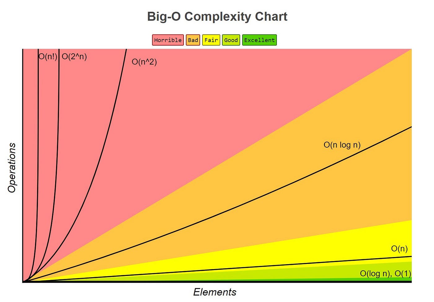
Complexities are ordered from fastest to slowest growth: O(1) < O(log n) < O(n) < O(n log n) < O(n²) < O(2ⁿ) < O(n!). Each class represents a different relationship between input size and the work an algorithm performs.
O(1) — Constant Time
The algorithm always takes the same amount of time regardless of input size. Accessing an array by index, hash map lookups, and push/pop on a stack are classic examples. Real-world analogy: looking up a word in a dictionary if you know the exact page number — you flip straight to it regardless of how thick the dictionary is.
o1_constant.py
python
# O(1) — Array index access
def get_first(arr):
    return arr[0]   # Always one operation, no matter how big arr is

# O(1) — Hash map lookup
def get_value(hashmap, key):
    return hashmap[key]   # Direct memory address calculation

# O(1) — Stack push / pop
stack = []
stack.append(42)    # O(1)
stack.pop()         # O(1)
O(log n) — Logarithmic Time
The algorithm halves the problem space at each step. Every time n doubles, the algorithm only does one extra step. Binary search is the textbook example. For n = 1,000,000,000, it only takes about 30 steps. Real-world analogy: finding a name in a phone book by repeatedly opening to the middle and discarding half.
binary_search.py
python
# O(log n) — Binary Search (array must be sorted)
def binary_search(arr, target):
    left, right = 0, len(arr) - 1

    while left <= right:
        mid = (left + right) // 2

        if arr[mid] == target:
            return mid
        elif arr[mid] < target:
            left = mid + 1    # Discard left half
        else:
            right = mid - 1   # Discard right half

    return -1

# Example
arr = [1, 3, 5, 7, 9, 11, 13, 15]
print(binary_search(arr, 7))   # → 3  (found at index 3)
print(binary_search(arr, 6))   # → -1 (not found)
O(n) — Linear Time
The algorithm visits each element once. Performance scales directly with input size. A single loop over an array is the classic case. Real-world analogy: checking every seat in a theater to find an empty one — the more seats, the longer it takes, proportionally.
linear_time.py
python
# O(n) — Find maximum value (one full pass)
def find_max(arr):
    max_val = arr[0]
    for item in arr:        # Visits every element exactly once
        if item > max_val:
            max_val = item
    return max_val

# O(n) — Linear search (unsorted array)
def linear_search(arr, target):
    for i, val in enumerate(arr):
        if val == target:
            return i
    return -1

# O(n) — Count occurrences
def count_occurrences(arr, target):
    return sum(1 for x in arr if x == target)
O(n log n) — Linearithmic Time
This is the complexity class of efficient sorting algorithms. It arises when you divide the problem into log n levels of recursion and do O(n) work at each level. It is also the proven lower bound for any comparison-based sorting algorithm. Algorithms in this class include Merge Sort, Heap Sort, and Quick Sort on average.
merge_sort.py
python
# O(n log n) — Merge Sort
def merge_sort(arr):
    if len(arr) <= 1:
        return arr

    mid   = len(arr) // 2
    left  = merge_sort(arr[:mid])    # Divide — log n levels
    right = merge_sort(arr[mid:])    # Divide — log n levels

    return merge(left, right)        # Conquer — O(n) per level

def merge(left, right):
    result, i, j = [], 0, 0
    while i < len(left) and j < len(right):
        if left[i] <= right[j]:
            result.append(left[i]); i += 1
        else:
            result.append(right[j]); j += 1
    result.extend(left[i:])
    result.extend(right[j:])
    return result

print(merge_sort([5, 3, 8, 1, 9, 2]))  # → [1, 2, 3, 5, 8, 9]
O(n²) — Quadratic Time
For every element, you look at every other element. A nested loop is the telltale sign. These algorithms become very slow quickly — 10x more data means 100x more work. For small inputs (n < 1,000), O(n²) is often acceptable and simpler to implement. For n > 10,000, prefer O(n log n) alternatives.
quadratic_time.py
python
# O(n²) — Bubble Sort
def bubble_sort(arr):
    n = len(arr)
    for i in range(n):                # Outer loop: n iterations
        for j in range(n - i - 1):    # Inner loop: up to n iterations
            if arr[j] > arr[j + 1]:
                arr[j], arr[j + 1] = arr[j + 1], arr[j]
    return arr

# O(n²) — Check all pairs for duplicates (naive approach)
def has_duplicates_naive(arr):
    for i in range(len(arr)):
        for j in range(i + 1, len(arr)):   # Every unique pair
            if arr[i] == arr[j]:
                return True
    return False

# O(n) alternative using a set — much better!
def has_duplicates_fast(arr):
    return len(arr) != len(set(arr))
O(2ⁿ) — Exponential Time
Adding one element to the input doubles the work. These algorithms explore every possible subset or combination. The naive recursive Fibonacci is a classic example — fib(50) makes roughly 2^50 calls, over one quadrillion. These are made practical with memoization (Dynamic Programming), which reduces Fibonacci to O(n) time and O(n) space.
exponential_vs_memo.py
python
# O(2ⁿ) — Naive Fibonacci (recomputes the same values over and over)
def fib(n):
    if n <= 1:
        return n
    return fib(n - 1) + fib(n - 2)   # Two recursive calls each time

# fib(6) generates this call tree:
#              fib(6)
#           /         \
#        fib(5)       fib(4)
#       /    \       /    \
#    fib(4) fib(3) fib(3) fib(2)   ...and so on

# O(n) — Fibonacci with memoization (each value computed once)
def fib_memo(n, memo={}):
    if n in memo:
        return memo[n]
    if n <= 1:
        return n
    memo[n] = fib_memo(n - 1, memo) + fib_memo(n - 2, memo)
    return memo[n]

print(fib(10))       # → 55  (slow for large n)
print(fib_memo(50))  # → 12586269025  (instant)
O(n!) — Factorial Time
The slowest practical complexity. The algorithm must evaluate every possible permutation of the input. The brute-force traveling salesman problem lives here. For n = 20, that is over 2 quintillion permutations. In practice, O(n!) algorithms are only feasible for n ≤ 10–12. For larger inputs, heuristics or approximation algorithms are used instead.
factorial_time.py
python
# O(n!) — Generate all permutations
from itertools import permutations

def all_permutations(arr):
    return list(permutations(arr))

print(all_permutations([1, 2, 3]))
# → [(1,2,3), (1,3,2), (2,1,3), (2,3,1), (3,1,2), (3,2,1)]
# n=3  →         6 permutations
# n=10 →   3,628,800 permutations
# n=20 →  2,432,902,008,176,640,000 permutations
Space Complexity
Big O applies to memory usage too, not just time. Space complexity measures how much extra memory an algorithm needs relative to input size. A key tradeoff in algorithm design is time vs space: memoization trades O(n) extra memory for a dramatic time improvement. Recursion also uses O(n) stack space proportional to the call depth, which can cause stack overflow for very large inputs.
space_complexity.py
python
# O(1) Space — In-place reversal, no extra memory allocated
def reverse_in_place(arr):
    left, right = 0, len(arr) - 1
    while left < right:
        arr[left], arr[right] = arr[right], arr[left]
        left  += 1
        right -= 1

# O(n) Space — Creates a brand new array of size n
def reverse_copy(arr):
    return arr[::-1]

# O(n) Space — n stack frames held in memory simultaneously
def factorial(n):
    if n == 0:
        return 1
    return n * factorial(n - 1)   # n calls deep on the call stack

# O(n) Space — Hash set to detect duplicates in O(n) time
def has_duplicates(arr):
    seen = set()          # Extra O(n) memory
    for x in arr:
        if x in seen:
            return True
        seen.add(x)
    return False
Best, Average & Worst Cases
Big O usually describes the worst case, but algorithms also have best and average cases. These are expressed with different notations: O(f(n)) is the upper bound or worst case, Ω(f(n)) is the lower bound or best case, and Θ(f(n)) is the tight bound or average case. Quick Sort is a great example: its average case is O(n log n), but degrades to O(n²) when the pivot is always the smallest or largest element, which happens on already-sorted input with naive pivot selection.
quicksort_cases.py
python
def quicksort(arr, low, high):
    if low < high:
        pivot_idx = partition(arr, low, high)
        quicksort(arr, low, pivot_idx - 1)
        quicksort(arr, pivot_idx + 1, high)

def partition(arr, low, high):
    pivot = arr[high]
    i = low - 1
    for j in range(low, high):
        if arr[j] <= pivot:
            i += 1
            arr[i], arr[j] = arr[j], arr[i]
    arr[i + 1], arr[high] = arr[high], arr[i + 1]
    return i + 1

# Best case:    O(n log n)  — pivot always splits array in half
# Average case: O(n log n)  — random pivot, balanced splits on average
# Worst case:   O(n²)       — pivot always smallest/largest (sorted input)
Amortized Analysis
Some operations are occasionally expensive but cheap on average. Dynamic arrays (like Python lists) are a classic example. Most appends are O(1) because space is already available. Occasionally an append triggers a resize and full copy, costing O(n). But amortized over n appends, the cost averages out to O(1) per operation — because each resize doubles the capacity, making the expensive copies increasingly rare.
amortized_append.py
python
# Python list append — amortized O(1)
items = []
for i in range(1_000_000):
    items.append(i)   # Occasionally O(n) for resize, O(1) on average

# Manual dynamic array to illustrate the concept
class DynamicArray:
    def __init__(self):
        self.data     = [None] * 1
        self.size     = 0
        self.capacity = 1

    def append(self, val):
        if self.size == self.capacity:   # Time to resize!
            self._resize()               # O(n) — happens rarely
        self.data[self.size] = val       # O(1) — happens most often
        self.size += 1

    def _resize(self):
        self.capacity *= 2               # Double the capacity
        new_data = [None] * self.capacity
        for i in range(self.size):
            new_data[i] = self.data[i]
        self.data = new_data
Big O Cheat Sheet
A quick reference for the time and space complexity of the most common data structures and sorting algorithms.
Sorting Algorithms at a Glance
Bubble Sort: Best O(n), Average O(n²), Worst O(n²), Space O(1). Insertion Sort: Best O(n), Average O(n²), Worst O(n²), Space O(1). Merge Sort: Best O(n log n), Average O(n log n), Worst O(n log n), Space O(n). Quick Sort: Best O(n log n), Average O(n log n), Worst O(n²), Space O(log n). Heap Sort: Best O(n log n), Average O(n log n), Worst O(n log n), Space O(1).
Data Structure Operations at a Glance
Array: Access O(1), Search O(n), Insert O(n), Delete O(n). Linked List: Access O(n), Search O(n), Insert O(1), Delete O(1). Hash Map: Access O(1) avg, Search O(1) avg, Insert O(1) avg, Delete O(1) avg. Binary Search Tree: All operations O(log n) average, O(n) worst. Heap: Peek O(1), Insert O(log n), Delete O(log n). Stack and Queue: Push/Enqueue O(1), Pop/Dequeue O(1).
Growth Rate Comparison at n = 1,000
O(1): 1 operation. O(log n): ~10 operations. O(n): 1,000 operations. O(n log n): ~10,000 operations. O(n²): 1,000,000 operations. O(2ⁿ): more operations than atoms in the observable universe — computationally impossible. O(n!): astronomically larger still — never feasible at this scale.
Related Links
Big-O Cheat Sheet
Visual reference for time and space complexity of common algorithms and data structures.
Introduction to Algorithms (CLRS)
The definitive textbook on algorithms — covers Big O rigorously with proofs and pseudocode.
Visualgo — Algorithm Visualizations
Interactive animations of sorting, searching, and graph algorithms to build intuition.
NeetCode — Algorithms & Interview Prep
Practical Big O explanations tied directly to coding interview problems.